Returns of financial stocks

Next, let’s choose the Dow Jones Industrial Average (DJIA) stocks and their ticker symbols and download some data. Besides the thirty stocks that make up the DJIA, we will also add SPY which is an SP500 ETF (Exchange Traded Fund).

We will use the rvest package to scrape the Wikipedia page for the constituents of DJIA

djia_url <- "https://en.wikipedia.org/wiki/Dow_Jones_Industrial_Average"


#get tables that exist on URL
tables <- djia_url %>% 
  read_html() %>% 
  html_nodes(css="table")


# parse HTML tables into a dataframe called djia. 
# Use purr::map() to create a list of all tables in URL
djia <- map(tables, . %>% 
               html_table(fill=TRUE)%>% 
               clean_names())


# constituents
table1 <- djia[[2]] %>% # the second table on the page contains the ticker symbols
  mutate(date_added = ymd(date_added),
         
         # if a stock is listed on NYSE, its symbol is, e.g., NYSE: MMM
         # We will get prices from yahoo finance which requires just the ticker
         
         # if symbol contains "NYSE*", the * being a wildcard
         # then we jsut drop the first 6 characters in that string
         ticker = ifelse(str_detect(symbol, "NYSE*"),
                          str_sub(symbol,7,11),
                          symbol)
         )

# we need a vector of strings with just the 30 tickers + SPY  + VIX
tickers <- table1 %>% 
  select(ticker) %>% 
  pull() %>% # pull() gets them as a sting of characters
  c("SPY", "^VIX") # and lets us add SPY, the SP500 ETF, and the VIX index

# Notice the cache=TRUE argument in the chunk options. Because getting data is time consuming, # cache=TRUE means that once it downloads data, the chunk will not run again next time you knit your Rmd

myStocks <- tickers %>% 
  tq_get(get  = "stock.prices",
         from = "2000-01-01") %>%
  group_by(symbol) 

glimpse(myStocks) # examine the structure of the resulting data frame

## Rows: 174,671
## Columns: 8
## Groups: symbol [32]
## $ symbol   <chr> "MMM", "MMM", "MMM", "MMM", "MMM", "MMM", "MMM", "MMM", "MMM"…
## $ date     <date> 2000-01-03, 2000-01-04, 2000-01-05, 2000-01-06, 2000-01-07, …
## $ open     <dbl> 48.0, 46.4, 45.6, 47.2, 50.6, 50.2, 50.4, 51.0, 50.7, 50.4, 4…
## $ high     <dbl> 48.2, 47.4, 48.1, 51.2, 51.9, 51.8, 51.2, 51.8, 50.9, 50.5, 4…
## $ low      <dbl> 47.0, 45.3, 45.6, 47.2, 50.0, 50.0, 50.2, 50.4, 50.2, 49.5, 4…
## $ close    <dbl> 47.2, 45.3, 46.6, 50.4, 51.4, 51.1, 50.2, 50.4, 50.4, 49.7, 4…
## $ volume   <dbl> 2173400, 2713800, 3699400, 5975800, 4101200, 3863800, 2357600…
## $ adjusted <dbl> 26.2, 25.1, 25.9, 27.9, 28.5, 28.3, 27.9, 27.9, 27.9, 27.5, 2…

Financial performance analysis depend on returns; If I buy a stock today for 100 and I sell it tomorrow for 101.75, my one-day return, assuming no transaction costs, is 1.75%. So given the adjusted closing prices, our first step is to calculate daily and monthly returns.

#calculate daily returns
myStocks_returns_daily <- myStocks %>%
  tq_transmute(select     = adjusted, 
               mutate_fun = periodReturn, 
               period     = "daily", 
               type       = "log",
               col_rename = "daily_returns",
               cols = c(nested.col))  

#calculate monthly  returns
myStocks_returns_monthly <- myStocks %>%
  tq_transmute(select     = adjusted, 
               mutate_fun = periodReturn, 
               period     = "monthly", 
               type       = "arithmetic",
               col_rename = "monthly_returns",
               cols = c(nested.col)) 

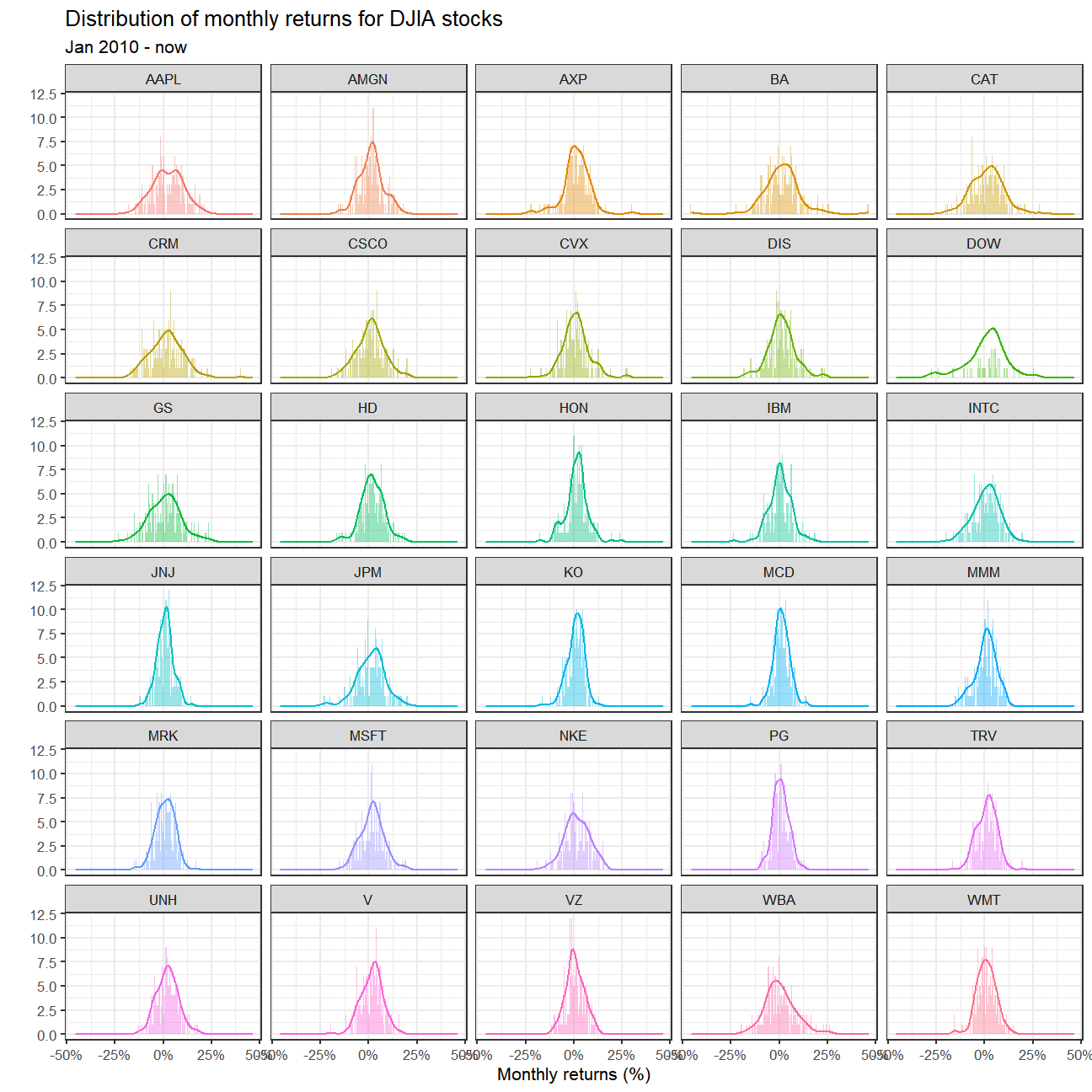
#visualise monthly returns since 2010, for each of the 30 DJIA stocks
myStocks_returns_monthly %>% 
  filter(symbol != "^VIX", symbol != "SPY") %>% 
  filter(date >= "2010-01-01") %>% 
  ggplot(aes(x = monthly_returns)) +
  geom_density(aes(colour = symbol), alpha = 1) +
  geom_histogram(aes(fill = symbol), alpha = 0.4, binwidth = 0.005)+
  facet_wrap(~symbol, nrow=7)+
  theme_bw(8)+
  theme(legend.position = "none") +
  scale_x_continuous(labels = scales::percent) +
  labs(
    title = "Distribution of monthly returns for DJIA stocks",
    subtitle = "Jan 2010 - now",
    x = "Monthly returns (%)",
    y = "" )+
  NULL